Supersonic plasma jets discovered

ESA - SWARM Mission logo.

23 March 2017

Information from ESA’s magnetic field Swarm mission has led to the discovery of supersonic plasma jets high up in our atmosphere that can push temperatures up to almost 10 000°C.

Presenting these findings at this week’s Swarm Science Meeting in Canada, scientists from the University of Calgary explained how they used measurements from the trio of Swarm satellites to build on what was known about vast sheets of electric current in the upper atmosphere.

Birkeland currents

The theory that there are huge electric currents, powered by solar wind and guided through the ionosphere by Earth’s magnetic field, was postulated more than a century ago by Norwegian scientist Kristian Birkeland.

It wasn’t until the 1970s, after the advent of satellites, however, that these ‘Birkeland currents’ were confirmed by direct measurements in space.

These currents carry up to 1 TW of electric power to the upper atmosphere – about 30 times the energy consumed in New York during a heatwave.

Upward and downward current sheets

They are also responsible for ‘aurora arcs’, the familiar, slow-moving green curtains of light that can extend from horizon to horizon.

While much is known about these current systems, recent observations by Swarm have revealed that they are associated with large electrical fields.

These fields, which are strongest in the winter, occur where upwards and downwards Birkeland currents connect through the ionosphere.

Heated ions travel upward

Bill Archer from the University of Calgary explained, “Using data from the Swarm satellites’ electric field instruments, we discovered that these strong electric fields drive supersonic plasma jets.

“The jets, which we call ‘Birkeland current boundary flows’, mark distinctly the boundary between current sheets moving in opposite direction and lead to extreme conditions in the upper atmosphere.

“They can drive the ionosphere to temperatures approaching 10 000°C and change its chemical composition. They also cause the ionosphere to flow upwards to higher altitudes where additional energisation can lead to loss of atmospheric material to space.”

Magnetic field sources

David Knudsen, also from the University of Calgary, added, “These recent findings from Swarm add knowledge of electric potential, and therefore voltage, to our understanding of the Birkeland current circuit, perhaps the most widely recognised organising feature of the coupled magnetosphere–ionosphere system.”

This discovery is just one of the new findings presented at the week-long science meeting dedicated to the Swarm mission. Also presented this week and focusing on Birkeland currents, for example, Swarm was used to confirm that these currents are stronger in the northern hemisphere and vary with the season.

Since they were launched in 2013, the identical Swarm satellites have been measuring and untangling the different magnetic signals that stem from Earth’s core, mantle, crust, oceans, ionosphere and magnetosphere.

Front of Swarm satellite

As well as a package of instruments to do this, each satellite has an electric field instrument positioned at the front to measure plasma density, drift and velocity.

Rune Floberghagen, ESA’s Swarm mission manager, said, “The electric field instrument is the first ionospheric imager in orbit so it’s very exciting to see such fantastic results that are thanks to this new instrument.

“The dedication of scientists working with data from the mission never ceases to amaze me and we are seeing some brilliant results, such as this, discussed at this week’s meeting.

“Swarm is really opening our eyes to the workings of the planet from deep down in Earth’s core to the highest part of our atmosphere.”

Related links:

ESA's Swarm: http://www.esa.int/Our_Activities/Observing_the_Earth/Swarm

Access Swarm data: https://earth.esa.int/web/guest/missions/esa-operational-eo-missions/swarm

Replay: Opening of Swarm and CryoSat Science Meetings: http://www.esa.int/spaceinvideos/Videos/2017/03/Opening_of_Swarm_and_CryoSat_Science_Meetings

Birkeland Centre for Space Science: https://birkeland.uib.no/

DTU Space: http://www.space.dtu.dk/english

University of Calgary–Physics and Astronomy: http://phas.ucalgary.ca/

Swarm–Aurora: https://swarm-aurora.com/

Images, Text, Credits: ESA/University of Calgary/DTU Space/ATG medialab.

Greetings, Orbiter.ch

BEAM Checks and Human Research Fill Crew Day & Astronauts Preparing for First of Three Spacewalks

ISS - Expedition 50 Mission patch.

March 22, 2017

The astronauts took a break from spacewalk preparations today and checked out an expandable module and worked on science freezers. The crew also continued its human research program exploring space nutrition and the effects of microgravity on metabolism and the immune system.

Thomas Pesquet opened the hatches to the Bigelow Expandable Activity Module (BEAM) today for a status check. The European Space Agency astronaut sampled BEAM’s air and surfaces for microbes and installed impact sensors. He also used a digital camera with a fish-eye lens to capture 360-degree imagery of the inside of BEAM.

Image above: This long-exposure photograph shows the docked Soyuz and Progress vehicles as the International Space Station orbits above the Earth. Image Credit: NASA.

Veteran NASA astronaut Peggy Whitson serviced three science freezers ensuring biological samples can be preserved for return on an upcoming SpaceX Dragon mission. She also brushed up on robotics skills necessary for Friday’s spacewalk.

Cosmonaut Oleg Novitskiy logged his meals again today before collecting saliva samples for an immunity study. Flight Engineer Andrey Borisenko researched how living in space long term affects metabolism and a crew member’s psychophysiological state.

Astronauts Preparing for First of Three Spacewalks

Three astronauts are preparing for a Friday morning spacewalk to upgrade and maintain the International Space Station’s external systems. The three cosmonauts stayed focused today on their set of Russian space experiments and life support work.

Astronauts Shane Kimbrough of NASA and Thomas Pesquet from the European Space Agency are reviewing procedures for the spacewalk set to begin Friday at 8 a.m. EDT with live NASA TV coverage at 6:30 a.m. NASA astronaut Peggy Whitson joined the pair for the review and will assist the spacewalkers from inside the station.

Image above: European Space Agency astronaut Thomas Pesquet is photographed during a spacewalk in January 2017. Image Credit: NASA.

Friday’s spacewalk will see Kimbrough and Pesquet begin setting up the station for future commercial crew missions. They will prepare the Pressurized Mating Adapter-3 for removal from the Tranquility module to the Harmony module. The astronauts will also replace computer relay boxes with software upgrades for future dockings of commercial crew vehicles.

In the midst of the spacewalk work today, Pesquet received a call from the French President Francois Hollande who toured an observatory with school children outside Lyon, France. Kimbrough and Whitson answered questions submitted by social media fans on Facebook Live Tuesday morning.

Related links:

Bigelow Expandable Activity Module (BEAM): https://www.nasa.gov/content/bigelow-expandable-activity-module

Immunity study: http://www.energia.ru/en/iss/researches/human/22.html

NASA TV: https://www.nasa.gov/multimedia/nasatv/index.html

Space Station Research and Technology: https://www.nasa.gov/mission_pages/station/research/index.html

International Space Station (ISS): https://www.nasa.gov/mission_pages/station/main/index.html

Images (mentioned), Text, Credits: NASA/Mark Garcia.

Best regards, Orbiter.ch

Sea Ice Extent Sinks to Record Lows at Both Poles

NASA - IceSat-2 Mission patch / NASA - Operation IceBridge patch.

March 22, 2017

Arctic sea ice appears to have reached on March 7 a record low wintertime maximum extent, according to scientists at NASA and the NASA-supported National Snow and Ice Data Center (NSIDC) in Boulder, Colorado. And on the opposite side of the planet, on March 3 sea ice around Antarctica hit its lowest extent ever recorded by satellites at the end of summer in the Southern Hemisphere, a surprising turn of events after decades of moderate sea ice expansion.

Arctic Sea Ice Reaches Another Record Low

Video above: The March 7, 2017, Arctic sea ice maximum extent was a record low, due to warmer-than-average temperatures, winds unfavorable to ice expansion, and a series of storms. Antarctic sea ice also broke a record with its annual minimum extent on March 3. Video Credits: NASA's Goddard Space Flight Center.

On Feb. 13, the combined Arctic and Antarctic sea ice numbers were at their lowest point since satellites began to continuously measure sea ice in 1979. Total polar sea ice covered 6.26 million square miles (16.21 million square kilometers), which is 790,000 square miles (2 million square kilometers) less than the average global minimum extent for 1981-2010 – the equivalent of having lost a chunk of sea ice larger than Mexico.

Graphic above: These line graphs plot monthly deviations and overall trends in polar sea ice from 1979 to 2017 as measured by satellites. The top line shows the Arctic; the middle shows Antarctica; and the third shows the global, combined total. The graphs depict how much the sea ice concentration moved above or below the long-term average. (They do not plot total sea ice concentration.) Arctic and global sea ice totals have moved consistently downward over 38 years. Antarctic trends are more muddled, but they do not offset the great losses in the Arctic. Graphic Credits: Joshua Stevens/NASA Earth Observatory.

The ice floating on top of the Arctic Ocean and surrounding seas shrinks in a seasonal cycle from mid-March until mid-September. As the Arctic temperatures drop in the autumn and winter, the ice cover grows again until it reaches its yearly maximum extent, typically in March. The ring of sea ice around the Antarctic continent behaves in a similar manner, with the calendar flipped: it usually reaches its maximum in September and its minimum in February.

This winter, a combination of warmer-than-average temperatures, winds unfavorable to ice expansion, and a series of storms halted sea ice growth in the Arctic. This year’s maximum extent, reached on March 7 at 5.57 million square miles (14.42 million square kilometers), is 37,000 square miles (97,00 square kilometers) below the previous record low, which occurred in 2015, and 471,000 square miles (1.22 million square kilometers) smaller than the average maximum extent for 1981-2010.

“We started from a low September minimum extent,” said Walt Meier, a sea ice scientist at NASA’s Goddard Space Flight Center in Greenbelt, Maryland. “There was a lot of open ocean water and we saw periods of very slow ice growth in late October and into November, because the water had a lot of accumulated heat that had to be dissipated before ice could grow. The ice formation got a late start and everything lagged behind – it was hard for the sea ice cover to catch up.”

Image above: On March 7, 2017, Arctic sea ice hit a record low wintertime maximum extent in 2017. At 5.57 million square miles, it is the lowest maximum extent in the satellite record, and 455,600 square miles below the 1981 to 2010 average maximum extent. Image Credits: NASA Goddard's Scientific Visualization Studio/L. Perkins.

The Arctic’s sea ice maximum extent has dropped by an average of 2.8 percent per decade since 1979. The summertime minimum extent losses are nearly five times larger: 13.5 percent per decade. Besides shrinking in extent, the sea ice cap is also thinning and becoming more vulnerable to the action of ocean waters, winds and warmer temperatures.

This year’s record low sea ice maximum extent might not necessarily lead to a new record low summertime minimum extent, since weather has a great impact on the melt season’s outcome, Meier said. “But it’s guaranteed to be below normal.”

In Antarctica, this year’s record low annual sea ice minimum of 815,000 square miles (2.11 million square kilometers) was 71,000 square miles (184,000 square kilometers) below the previous lowest minimum extent in the satellite record, which occurred in 1997.

Antarctic sea ice saw an early maximum extent in 2016, followed by a very rapid loss of ice starting in early September. Since November, daily Antarctic sea ice extent has continuously been at its lowest levels in the satellite record. The ice loss slowed down in February.

Image above: On March 3, 2017, the sea ice cover around the Antarctic continent shrunk to its lowest yearly minimum extent in the satellite record, in a dramatic shift after decades of moderate sea ice expansion. Image Credits: NASA Goddard's Scientific Visualization Studio/L. Perkins.

This year’s record low happened just two years after several monthly record high sea ice extents in Antarctica and decades of moderate sea ice growth.

“There’s a lot of year-to-year variability in both Arctic and Antarctic sea ice, but overall, until last year, the trends in the Antarctic for every single month were toward more sea ice,” said Claire Parkinson, a senior sea ice researcher at Goddard. “Last year was stunningly different, with prominent sea ice decreases in the Antarctic. To think that now the Antarctic sea ice extent is actually reaching a record minimum, that’s definitely of interest.”

Image above: Operation IceBridge, NASA’a aerial survey of polar ice, flies over a lead, or opening in the sea ice cover, near the Alaskan coast on March 11, 2017. Image Credits: NASA/Jeremy Harbeck.

Meier said it is too early to tell if this year marks a shift in the behavior of Antarctic sea ice.

“It is tempting to say that the record low we are seeing this year is global warming finally catching up with Antarctica,” Meier said. “However, this might just be an extreme case of pushing the envelope of year-to-year variability. We’ll need to have several more years of data to be able to say there has been a significant change in the trend.”

Related links:

NSIDC announcement: http://nsidc.org/arcticseaicenews/2017/03/arctic-sea-ice-maximum-at-record-low/

Data visualization: Minimum Antarctic Sea Ice 2017: https://svs.gsfc.nasa.gov/4562

Data visualization: Arctic Daily Sea Ice Concentration from Arctic Minimum 2016 to Arctic Maximum 2017: https://svs.gsfc.nasa.gov/4564
    
"2016 Arctic Sea Ice Wintertime Extent Hits Another Record Low" (March 28, 2016): https://www.nasa.gov/feature/goddard/2016/2016-arctic-sea-ice-wintertime-extent-hits-another-record-low

"NASA Study Shows Global Sea Ice Diminishing, Despite Antarctic Gains" (Feb. 10, 2015): https://www.nasa.gov/content/goddard/nasa-study-shows-global-sea-ice-diminishing-despite-antarctic-gains

"Arctic Sea Ice Annual Minimum Ties Second Lowest on Record" (Sept. 15, 2016): https://www.nasa.gov/feature/goddard/2016/arctic-sea-ice-annual-minimum-ties-second-lowest-on-record

ICESat-2: http://www.nasa.gov/content/goddard/icesat-2

IceBridge: http://www.nasa.gov/mission_pages/icebridge/index.html

Images (mentioned), Video (mentioned), Text, Credits: NASA's Earth Science News Team, by Maria-José Viñas/Rob Garner.

Greetings, Orbiter.ch

NASA Taking First Steps Toward High-speed Space ‘Internet’

NASA - Space Communications and Navigation (SCaN) logo.

March 22, 2017

NASA is developing a trailblazing, long-term technology demonstration of what could become the high-speed internet of the sky.

The Laser Communications Relay Demonstration (LCRD) will help NASA understand the best ways to operate laser communications systems. They could enable much higher data rates for connections between spacecraft and Earth, such as scientific data downlink and astronaut communications.

Animation above: Conceptual animation depicting a satellite using lasers to relay data from Mars to Earth. Animation Credits: NASA's Goddard Space Flight Center.

“LCRD is the next step in implementing NASA’s vision of using optical communications for both near-Earth and deep space missions,” said Steve Jurczyk, associate administrator of NASA’s Space Technology Mission Directorate, which leads the LCRD project. “This technology has the potential to revolutionize space communications, and we are excited to partner with the Human Exploration and Operations Mission Directorate’s Space Communications and Navigation program office, MIT Lincoln Labs and the U.S. Air Force on this effort.”

Laser communications, also known as optical communications, encodes data onto a beam of light, which is then transmitted between spacecraft and eventually to Earth terminals. This technology offers data rates that are 10 to 100 times better than current radio-frequency (RF) communications systems. Just as important, laser communication systems can be much smaller than radio systems, allowing the spacecraft communication systems to have lower size, weight and power requirements. Such capability will become critically important as humans embark on long journeys to the moon, Mars and beyond.

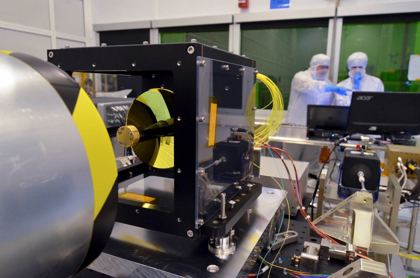
Image above: An engineer examines the gimbal and latch assembly component of one of LCRD’s two optical module assembly. The optical module, when combined with the modems and controller electronics, make up the LCRD’s flight payload. Image Credits: NASA's Goddard Space Flight Center/Sandra Vilevac.

“LCRD is designed to operate for many years and will allow NASA to learn how to optimally use this disruptive new technology,” said Don Cornwell, director of the  Advanced Communication and Navigation division of the Space Communications and Navigation program office at NASA Headquarters, which leads the development of the instrument. “We are also designing a laser terminal for the International Space Station that will use LCRD to relay data from the station to the ground at gigabit-per-second data rates. We plan to fly this new terminal in 2021, and once tested, we hope that many other Earth-orbiting NASA missions will also fly copies of it to relay their data through LCRD to the ground.”

The mission builds upon the Lunar Laser Communications Demonstration (LLCD), a very successful pathfinder mission that flew aboard the Lunar Atmosphere Dust and Environment Explorer in 2013. While LLCD was first to demonstrate high-data-rate laser communications beyond low-Earth orbit, LCRD will demonstrate the technology’s operational longevity and reliability. The mission will also test LCRD’s capabilities within many different environmental conditions and operational scenarios.

Image above: Engineers are currently testing the optical module assemblies on the Goddard-built optical test bench to ensure pointing accuracy during the upcoming mission. Image Credits: NASA's Goddard Space Flight Center/Sandra Vilevac.

“We’ve learned a lot over the years about radio-frequency communications and how it works to make the most of the technology,” Dave Israel, LCRD’s principal investigator, said about the current communications system. “With LCRD, we’ll have the opportunity to put laser communications through its paces to test the performance over different weather conditions and times of day to get that experience.”

LCRD is designed to function between two and five years. Two ground terminals equipped with laser modems located in Table Mountain, California, and in Hawaii will demonstrate communications capability to and from LCRD, which will be located in an orbit that matches Earth's rotation, called a geosynchronous orbit, between the two stations.

The LCRD payload consists of two identical optical terminals connected by a component called a space switching unit, which acts as a data router. The space switching unit is also connected to a radio-frequency downlink.

The modems translate digital data into laser or radio-frequency signals and back again. Once they convert the data to laser light, the optical module will beam the data to Earth. To do so, the module must be perfectly pointed to receive and transmit the data. The controller electronics (CE) module commands actuators to help point and steady the telescope despite any movement or vibration on the spacecraft.

LCRD recently successfully passed a key decision point review and has moved on to the integration and test stage of development, during which engineers will ensure each component will behave as intended after the instrument launches. Launch is scheduled to occur in summer 2019.

The LCRD team is led by NASA’s Goddard Space Flight Center in Greenbelt, Maryland. Partners include NASA’s Jet Propulsion Laboratory in Pasadena, California, and MIT’s Lincoln Laboratory.

LCRD is a project within NASA's Space Technology Mission Directorate’s Technology Demonstration Mission, which performs system level demonstrations of cross-cutting technologies and capabilities and bridges the gap between scientific and engineering challenges and the technological innovations needed to overcome them, enabling robust new space missions like LCRD.

For more information about NASA’s Technology Demonstration Mission, visit:

https://www.nasa.gov/mission_pages/tdm/main/index.html

The Space Communications and Navigation (SCaN) program office at NASA Headquarters in Washington provides strategic and programmatic oversight to enable the mission. These capabilities form the backbone of all NASA missions, including LCRD, providing critical connectivity from spacecraft to ground.

For more information about SCaN, visit: https://www.nasa.gov/directorates/heo/scan/index.html

Related links:

Laser Communications Relay Demonstration (LCRD): https://esc.gsfc.nasa.gov/lcrd

Lunar Laser Communications Demonstration (LLCD): https://www.nasa.gov/content/goddard/historic-demonstration-proves-laser-communication-possible

Animation (mentioned), Images (mentioned), Text, Credits: NASA’s Goddard Space Flight Center, by Ashley Hume/Rob Garner.

Best regards, Orbiter.ch

Ice in Ceres' Shadowed Craters Linked to Tilt History

NASA - Dawn Mission patch.

March 22, 2017

Dwarf planet Ceres may be hundreds of millions of miles from Jupiter, and even farther from Saturn, but the tremendous influence of gravity from these gas giants has an appreciable effect on Ceres' orientation. In a new study, researchers from NASA's Dawn mission calculate that the axial tilt of Ceres -- the angle at which it spins as it journeys around the sun -- varies widely over the course of about 24,500 years. Astronomers consider this to be a surprisingly short period of time for such dramatic deviations.

Animation above: This animation shows how the illumination of Ceres' northern hemisphere varies with the dwarf planet's axial tilt, or obliquity. Shadowed regions are highlighted for tilts of 2 degrees, 12 degrees and 20 degrees. Animation Credits: NASA/JPL-Caltech/UCLA/MPS/DLR/IDA.

Changes in axial tilt, or "obliquity," over the history of Ceres are related to the larger question of where frozen water can be found on Ceres' surface, scientists report in the journal Geophysical Research Letters. Given conditions on Ceres, ice would only be able to survive at extremely cold temperatures -- for example, in areas that never see the sun.

"We found a correlation between craters that stay in shadow at maximum obliquity, and bright deposits that are likely water ice," said Anton Ermakov, postdoctoral researcher at NASA's Jet Propulsion Laboratory, Pasadena, California, and lead author of the study. "Regions that never see sunlight over millions of years are more likely to have these deposits."

Cycles of Obliquity

Throughout the last 3 million years, Ceres has gone through cycles where its tilt ranges from about 2 degrees to about 20 degrees, calculations indicate.

"We cannot directly observe the changes in Ceres’ orientation over time, so we used the Dawn spacecraft’s measurements of shape and gravity to precisely reconstruct what turned out to be a dynamic history," said Erwan Mazarico, a co-author at NASA's Goddard Space Flight Center in Greenbelt, Maryland.

The last time the dwarf planet reached a maximum tilt, which was about 19 degrees, was 14,000 years ago, researchers said. For comparison, Earth is tilted 23.5 degrees. This significant tilt causes our planet to experience seasons: The northern hemisphere experiences summer when it is oriented toward the sun, and winter when it's pointed away from the sun. By contrast, Ceres' current tilt is about 4 degrees, so it will not have such strong seasonal effects over the course of a year there (which is about 4.6 Earth years).

How Obliquity Relates to Ice

When the axial tilt is small, relatively large regions on Ceres never receive direct sunlight, particularly at the poles. These persistently shadowed regions occupy an area of about 800 square miles (2,000 square kilometers). But when the obliquity increases, more of the craters in the polar regions receive direct exposure to the sun, and persistently shadowed areas only occupy 0.4 to 4 square miles (1 to 10 square kilometers). These areas on Ceres' surface, which stay in shadow even at high obliquity, may be cold enough to maintain surface ice, Dawn scientists said.

These craters with areas that stay in shadow over long periods of time are called "cold traps," because they are so cold and dark that volatiles -- substances easily vaporized -- that migrate into these areas can’t escape, even over a billion years. A 2016 study by the Dawn team in Nature Astronomy found bright material in 10 of these craters, and data from Dawn's visible and infrared mapping spectrometer indicate that one of them contains ice.

The new study focused on polar craters and modeled how shadowing progresses as Ceres' axial tilt varies. In the northern hemisphere, only two persistently shadowed regions remain in shadow at the maximum 20-degree tilt. Both of these regions have bright deposits today. In the southern hemisphere, there are also two persistently shadowed regions at highest obliquity, and one of them clearly has a bright deposit.

Shadowed Regions in Context

Ceres is the third body in the solar system found to have permanently shadowed regions. Mercury and Earth's moon are the other two, and scientists believe they received their ice from impacting bodies. However, Mercury and the moon do not have such wide variability in their tilts because of the stabilizing gravitational influence of the sun and Earth, respectively. The origin of the ice in Ceres' cold traps is more mysterious -- it may come from Ceres itself, or may be delivered by impacts from asteroids and comets. Regardless, the presence of ice in cold traps could be related to a tenuous water atmosphere, which was detected by ESA's Herschel Space Observatory in 2012-13. Water molecules that leave the surface would fall back onto Ceres, with some landing in cold traps and accumulating there. 

"The idea that ice could survive on Ceres for long periods of time is important as we continue to reconstruct the dwarf planet's geological history, including whether it has been giving off water vapor," said Carol Raymond, deputy principal investigator of the Dawn mission and study co-author, based at JPL.

Artist's view of the Dawn spacecraft flyby. Image Credits: NASA/JPL

Dawn's mission is managed by JPL for NASA's Science Mission Directorate in Washington. Dawn is a project of the directorate's Discovery Program, managed by NASA's Marshall Space Flight Center in Huntsville, Alabama. UCLA is responsible for overall Dawn mission science. Orbital ATK Inc., in Dulles, Virginia, designed and built the spacecraft. The German Aerospace Center, Max Planck Institute for Solar System Research, Italian Space Agency and Italian National Astrophysical Institute are international partners on the mission team. For a complete list of mission participants, visit:

http://dawn.jpl.nasa.gov/mission

More information about Dawn is available at the following sites:

http://dawn.jpl.nasa.gov

http://www.nasa.gov/dawn

Image (mentioned), Animation (mentioned), Text, Credits: NASA/Tony Greicius/JPL/Elizabeth Landau.

Greetings, Orbiter.ch

NASA’s SDO Sees a Stretch of Spotless Sun

NASA - Solar Dynamics Observatory (SDO) patch.

March 22, 2017

For 15 days starting on March 7, 2017, NASA’s Solar Dynamics Observatory, or SDO, returned visible light images of a yolk-like spotless sun. This is the longest stretch of spotlessness since the last solar minimum in April 2010, indicating the solar cycle is marching on toward the next minimum, which scientists predict will occur between 2019—2020.

The sun goes through a natural 11-year cycle marked by two extremes: solar maximum and solar minimum. Sunspots are dark regions of complex magnetic activity on the sun’s surface, so the number of sunspots at any given time is used as an index for solar activity. Solar maximum is characterized by intense solar activity and the greatest sunspot number. Conversely, during solar minimum, the sun is least active and sunspot number is at its lowest. Solar activity, however, does not end as sunspot number decreases toward minimum. There are other sources of solar activity such as high-speed streams of solar material from coronal holes, which spark aurora and other space weather effects.

Solar Dynamics Observatory (SDO). Image Credits: NASA/JPL

The SDO images here compare the sun on March 20, 2017, and February 27, 2014, during the last solar maximum when the sun sported numerous spots.

NASA's SDO (Solar Dynamics Observatory): http://www.nasa.gov/mission_pages/sdo/main/index.html

Image (mentioned), Animation (mentioned), Text, Credits: NASA’s Goddard Space Flight Center, by Lina Tran/Lynn Jenner.

Greetings, Orbiter.ch

Swarm detects asymmetry

ESA - SWARM Mission logo.

22 March 2017

Strong electric currents in the upper atmosphere are known to vary according to the season, but ESA’s Swarm mission has discovered that this seasonal variation is not the same in the north and south polar regions.

Named after Kristian Birkeland, the scientist a century ago who first postulated that the ‘northern lights’ were linked to electrically charged particles in the solar wind, these currents flow along Earth’s magnetic field lines in the polar regions.

Seasonal asymmetry

Magnetic field measurements from ESA’s Swarm satellite constellation are allowing scientists to understand more about these powerful currents, which carry up to 1 TW of electric power to the upper atmosphere. This is about 30 times the energy consumed in New York during a heatwave.

It is important to understand the interplay between these Birkeland currents and the solar wind that bombards our planet and that can potentially cause power and communication blackouts.

New findings, presented this week at the Swarm science meeting in Canada, show how three years of measurements from the mission were combined with measurements from Germany’s earlier Champ satellite to produce global climatological maps of these currents.

Moreover, these results show differences between currents in the northern and southern hemisphere, how they change with the season and how they vary according to the strength of the solar wind.

Earth's protective shield

Karl Laundal, from the Birkeland Centre for Space Science, explained, “Interaction between Earth’s magnetic field and the interplanetary magnetic field – meaning part of the Sun’s magnetic field carried by solar wind – depends on how the interplanetary field is orientated.

“While this sounds complicated, it means that hardly any solar wind can enter the magnetosphere and arrive at Earth if the interplanetary magnetic field points north, parallel to Earth’s magnetic field.

“On the other hand, if the interplanetary field points south, the opposite is true and this allows a connection to be made with Earth’s magnetic field.

“Part of the energy in solar wind then further energises the charged particles that are responsible for the visible light displays of the auroras.”

Birkeland currents therefore tend to be weak for a northwards interplanetary field and strong for a southwards field.

 Swarm

Importantly, these new results also reveal that the strength of the currents is not the same in both hemispheres. These hemispheric differences may relate to asymmetry in Earth’s main magnetic field.

In fact, the two geomagnetic poles are not geometrically opposite to one another, and the magnetic field intensity is also not the same in the north as in the south.

Dr Laundal said, “The main reason for this probably has to do with differences in Earth’s main field. Such differences imply that the ionosphere–magnetosphere coupling is different in the two hemispheres.

Asymmetry detail

“In particular, the magnetic pole is more offset with respect to the geographic pole in the south compared to north, which leads to different variations in sunlight in the ‘magnetic hemispheres’. Because of these differences, the two hemispheres do not respond symmetrically to solar wind driving or changing seasons.

“Swarm is a fantastic tool for space science studies. The high-quality measurements and the fact that there are three satellites working in concert hold many new clues about how our home planet interacts with the space around it. It’s a fascinating time.”

Related links:

ESA's Swarm: http://www.esa.int/Our_Activities/Observing_the_Earth/Swarm

Access Swarm data: https://earth.esa.int/web/guest/missions/esa-operational-eo-missions/swarm

Replay: Opening of Swarm and CryoSat Science Meetings: http://www.esa.int/spaceinvideos/Videos/2017/03/Opening_of_Swarm_and_CryoSat_Science_Meetings

Birkeland Centre for Space Science: https://birkeland.uib.no/

DTU Space: http://www.space.dtu.dk/english

University of Calgary–Physics and Astronomy: http://phas.ucalgary.ca/

CHAMP: http://op.gfz-potsdam.de/champ/

Images, Text, Credits: ESA/DTU/BCSS/ATG medialab.

Greetings, Orbiter.ch